Ham TestHere come some tests that could be of interest for HAM operators.
First, I should ensure that expectations don’t get unrealistic. A general-purpose oscilloscope like the SDS800X HD is neither a spectrum analyzer nor a test receiver, even when its noise figure drops below 10 dB at frequencies above 300 kHz. Yet it just works on the full input signal bandwidth, there is no pre-selector, no mixer to shift small portions of the upper spectrum down to a lower intermediate frequency and no filter that could isolate the IF signal.
In the time domain, 400 µVrms is pretty much the limit for reliable triggering, indicated by a correct trigger frequency counter display; for even lower levels, triggering gets increasingly sporadic and at 100 µVrms, the trigger frequency counter drops below 1 MHz. Only if we have a strong copy of the signal of interest, such as measuring the stop band of a filter, we could trigger on the input signal and use the Average math function to make even very weak output signals visible and measurable, even those way below the noisefloor, as has been demonstrated already in this thread.
For all the following tests, a Siglent SDG7102A AWG with OCXO option has been directly connected with coaxial Hyperflex 5 cables, a step-attenuator Wavetek 5080.1 and an inline terminator “hp10100C” at the scope input.
CW TestFor the 1 mVrms demo I had to bring quite a lot of information onto a single screen:
SDS824X HD_SA_CW_146MHz_1mV
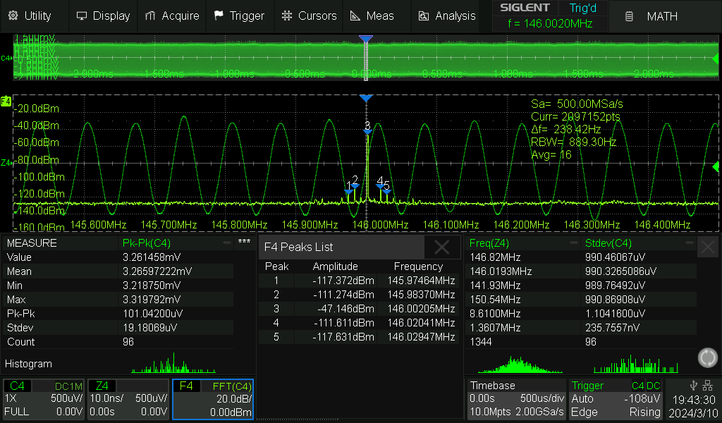
The main window at the top is showing the 146 MHz signal at a timebase of 500 µs/div. We need that slower timebase to get sufficient data for a 2 Mpts FFT. Of course we can’t see any details there, hence there is the zoom window below, where the signal is displayed at a timebase of 10 ns/div. We can see that the vertical position is not constant across the screen width, which hints on the noise that gets very noticeable at such low signal levels.
The zoom window also contains the FFT which reveals some weak modulation due to noise and we can see the corresponding sidebands indicated by markers 1, 2, 4 and 5, whereas marker 3 corresponds to the main signal.
Below we have two windows nested: the advanced measurements together with the Peaks List, for which I’ve freed up some space by removing measurements 2 and 3. We can see that the amplitude measurements in the time domain still work reasonably well, at least Stdev (= AC-RMS), whereas the peak-to-peak amplitude cannot be accurate – once again because of the noise.
The signal frequency measurement is not accurate as well and all automatic measurements have a high variance, as can be seen in the measurement statistics and histograms, yet the 7-digit trigger frequency counter is still rock stable and pretty accurate. Of course, it is 2 kHz off, which is equivalent to 13.7 ppm, but that’s because the time base of the SDS800X HD has 25 ppm tolerance, which is pretty much standard, while Siglent’s higher end DSOs starting at the SDS2000X plus provide class leading 1 ppm timebase accuracy.
The peak table shows the various signal amplitudes, but we are mainly interested in Peak #3, which is indicated as -47.146 dBm at 146.00205 MHz. Surprisingly, the frequency is exactly the same as the trigger frequency counter, hence absolutely correct relative to the SDS800X HD timebase, also the amplitude is pretty much spot on (should ideally be -47.0 dBm).
At this point I should mention that the Peak table is automatic and we only set the search parameters, i.e. threshold and excursion. This is in contrast to the Markers, which can be preset on peaks or harmonics, yet each marker can be set individually to any desired frequency by the user. For the measurements here, Peak tables have been used exclusively.
There is no point to further look at the time domain for weaker signals, because they will get heavily distorted and eventually buried in the noise anyway. Yet I don’t change the arrangement and only move the zoom trace out of view.
Next, we try 100 µVrms:
SDS824X HD_SA_CW_146MHz_100uV
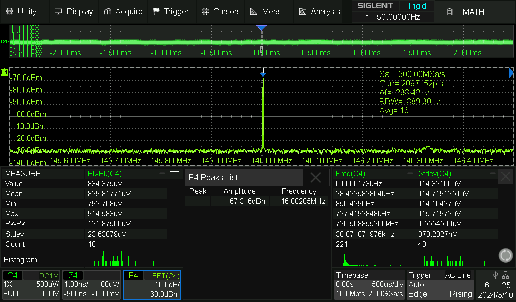
The main window at the top shows mainly noise for the 100 µVrms signal at 245 MHz bandwidth. The zoom window with the FFT displays a clean spectral line, hence we only get a single peak marker.
The advanced measurements below just try to measure the noise, even though the Stdev measurement still isn’t too far off – just a coincidence?
Since such a weak signal cannot be properly triggered anymore anyway, I’ve used AC-line trigger instead and the trigger frequency counter just shows a constant 50 Hz now. FFT doesn’t need a triggered signal.
The peak table shows the signal amplitude as -67.316 dBm at 146.00205 MHz. The amplitude is still pretty accurate (should ideally be -67.0 dBm).
Now let’s try 10 µVrms:
SDS824X HD_SA_CW_146MHz_10uV
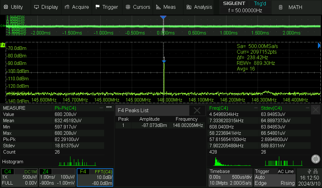
Once again, we get a clean spectral line with a single peak marker.
The advanced measurements below are totally meaningless, but the peak table shows the signal amplitude extremely accurate as -87.073 dBm at 146.00205 MHz.
Another attempt with 1 µVrms:

SDS824X HD_SA_CW_146MHz_1uV
One more time, we get a clean spectral line with a single peak marker.
The advanced measurements below are totally meaningless, but the peak table shows the signal amplitude pretty accurately as -107.291 dBm at 146.00205 MHz.
A final attempt with 100 nVrms:
SDS824X HD_SA_CW_146MHz_100nV
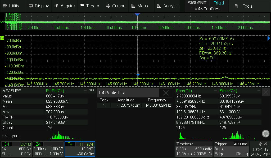
We even get a tiny spectral line, but have to tweak the search parameters to get the peak marker. Its amplitude is now way off: -123.737 dBm at 146.00182 MHz (should be -127.0 dBm). The signal is just too close to the noise floor now.
This test is quite revealing. Even a 100 nVrms signal could be detected, and even though the signal amplitude was off by 3.26 dB, the frequency could still be measured with just ~200 Hz error (relative to the DSO’s timebase that is)!
FM TestFor the modulation tests, I did not feel like trying many different levels again, so 1 mV and 10 µV RMS shall be sufficient for FM.
First I need to repeat what I’ve already stated initially: An oscilloscope is a baseband instrument, not a spectrum analyzer. There is only so much frequency resolution we can get from a 2 Mpts FFT. As a consequence, the expectations shouldn’t be very high when looking at one kilohertz frequency spacing in signals from the 2 meter band.
Modulation: 1 kHz modulation frequency and 5 kHz frequency deviation.
1 mVrms at 146 MHz first:

SDS824X HD_SA_FM_146MHz_1mV
Well, that’s not very convincing. I was forced to use the Blackman window, which is still usable for spectrum analysis with a max. amplitude error of 1 dB. Its resolution bandwidth is not that much better than Flattop hence the picture isn’t very useful and we only get a vague idea of the FM spectrum.
It should be clear that a general-purpose oscilloscope isn’t a test receiver. If we look at bandwidth limited signals, like filtered IF, where we need not worry about aliasing from unrelated signals in the neighborhood, we could just use the “frequency conversion by undersampling” method.
Any ADC acts as a mixer, thus producing a spectrum of ±
n *
fi ±
m *
fs, where
fi is the input frequency and
fs is the sample clock, while
n and
m are just integers running from 0 to (theoretically) infinity. During normal operation, we don’t want to see any mixer products, which is perfectly possible as long as the input signal and all its harmonics don’t exceed
fs/2 and the output of the ADC has a brick-wall filter (then in the digital domain of course, aka Sinc filter or sin(x)/x reconstruction) that removes everything above
fs/2.
Yet in some circumstances, we can make use of a certain high-order mixer product, just as in this example, where the effective FFT sample rate is only 5 MSa/s, which is quite obviously way too low for a 146 MHz input signal.
According to the formula given above, we are aiming at the mixer product for 1 *
fi - 29 *
fs, which is
1 * 146 MHz – 29 x 5 MHz = 146 MHz – 145 MHz = 1 MHz;
Now if we set the center frequency to 1 MHz, we get the carrier at 146 MHz and a resolution bandwidth of only 35.57 Hz, even with just 512 kpts FFT, hence can also clearly see the sidebands and their 1 kHz spacing. 16x averaging has been used in order to get a clean and stable display:

SDS824X HD_SA_FM_146MHz_1mV_5MSa
Be aware that the true center frequency is Peak #6 at 1.00197 MHz because of the SDS824X HD timebase tolerance of 25 ppm.
The following table compares the measured sidebands with the expected ones in dBm:
Ord. Meas. Expected
0 -62.052 -62.083
1 -56.750 -56.763
2 -73.700 -73.713
3 -55.823 -55.833
4 -55.200 -55.223
Now for the 10 µVrms test:
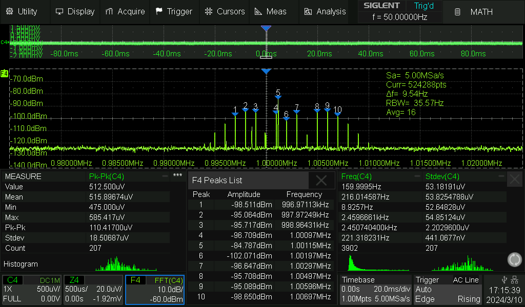
SDS824X HD_SA_FM_146MHz_10uV_5MSa
There is a spurious signal at marker 5 exceeding the signal spectrum – we just have to ignore it.
The following table compares the measured sidebands with the expected ones in dBm:
Ord. Meas. Expected
0 -102.07 -102.083
1 -96.700 -96.763
2 -113.70 -113.713
3 -95.700 -95.833
4 -95.100 -95.223
5 -98.500 -98.733
All in all the down-mixing via the ADC can save our day as long as we have an isolated signal and the signal levels don’t get too low.
There are several caveats though:
• We need to make sure that
n is always positive, otherwise we’d get the result in reverse frequency position, i.e. the upper sideband appears below the carrier and vice versa.
• Mixing with the 29th harmonic of the sample clock introduces also 29 times more phase noise and jitter and this might get visible the FFT plot.
• Amplitude accuracy might suffer, as a harmonic mixing process is not guaranteed to be as efficient as the fundamental one, hence we might see some attenuation.
AM TestModulation: 1 kHz modulation frequency and 80% modulation depth.

SDS824X HD_SA_AM_146MHz_1mV
Well, that looks familiar. Once again, the picture isn’t great and we only get a vague idea of the AM spectrum. The sidebands should be -8 dBc = -61.6 dBm. The deviations come from the insufficient resolution bandwidth and the amplitude error of the Blackman window.
We are looking at the mixer product for 1 *
fi - 29 *
fs again, which is
1 * 146 MHz – 29 x 5 MHz = 146 MHz – 145 MHz = 1 MHz;
Now if we set the center frequency to 1 MHz, we get the carrier at 146 MHz and a resolution bandwidth of only 35.57 Hz, hence can also clearly see the sidebands and their 1 kHz spacing. 16x averaging has been used in order to get a clean and stable display:

SDS824X HD_SA_FM_146MHz_1mV_5MSa
Be aware that the true center frequency is Peak #3 at 1.00197 MHz because of the SDS824X HD timebase tolerance.
The sidebands should be -8 dBc = -55 dBm. The accuracy is very high despite the harmonic mixing process.
General Remark: I don’t maintain a YouTube channel and my time is limited. Since I’ve already published most of the intended content, and I made sure the relevant information can easily be found by means of the table of contents in the opening posting, I don’t mind people asking questions here, even newbie questions 😉
EDIT: Corrected the statement for the 10 µV FM-test and added a comparison of measured vs. expected results.


