Somebody has been spending a lot of quality time with LTspice! That is some very slick work.
Glad you like it, thank you

, though it was offtopic because OP was asking for Octave/Matlab code to FFT -> filter -> iFFT.
After seeing the big oscillations from the OP screen captures, I was curious how much of it could be caused by the worst filter (worst as in the most abrupt, but not self oscillating IIR), so here's the Octave code and attached plots for a brick low pass filter.
The test square signal (14MHz/10ns on) was FFT-ed first, then every spectral component above the F
cut of the presumed low pass filter was removed, then iFFT to reconstruct the display trace:
F_cut(1) = 150_000_000;  # 150MHz MUST be declared from hightest to lowest
F_cut(2) = 100_000_000;  # 100MHz
F_cut(3) =  50_000_000;  #  50MHz

L = 1000;  # number of samples to consider
Fs = 1_000_000_000;  # 1GSa/s sampling
Ts = 1/Fs;
t = (0:L-1)*Ts;

F_tst = 14_000_000;  # 14 MHz square wave test signal
T_tst_on = 10e-9; # 10ns square wave level high duration
T_tst_all = 1/F_tst;


# generate the test signal waveform Sig_tst
Sig_tst(1) = 0;  # start from 0V
for i = 2:L;
    time = (i-1)*Ts;
    if (mod(time, T_tst_all) <= T_tst_on)
      Sig_tst(i) = 4.8;  # Test signal level is 4.8V
    else
      Sig_tst(i) = 0;   # Test signal level is 0V
    endif
endfor


# plot the test signal (only the first 100 samples for clarity)
subplot(2, 2, 1);
set(gca, 'FontSize', 20)
hold on
plot(1_000_000_000*t(1:100), Sig_tst(1:100), 'b', 'linewidth', 3)
#plot(1_000_000_000*t, Sig_tst)
title ('Test signal')
xlabel('t (ns)')
ylabel('Test signal (V)')

# double sided FFT
Y = fft(Sig_tst);


# plot single sided spectrum
P2 = abs(Y/L);
P1 = P2(1:L/2+1);
P1(2:end-1) = 2*P1(2:end-1);

f = Fs*(0:(L/2))/L;

subplot(2, 2, 2);
set(gca, 'FontSize', 20)
hold on
plot(f/1_000_000, P1, 'b', 'linewidth', 3)
title('Single-sided spectrum of the test signal')
xlabel('f (MHz)')
ylabel('Spectral amplitude')


# brick low pass filter F_cut(1)
for bin = 1:L
  if bin <= L/2
    F_bin = (bin-1)*Fs/L;
  else
    F_bin = (L-bin+1)*Fs/L;
  endif
  if F_bin > F_cut(1)
    Y(bin) = 0;
  endif;
endfor;

# back to time domain
Sig_DSP = ifft(Y);

subplot(2, 2, 3);
set(gca, 'FontSize', 20)
hold on
plot(1_000_000_000*t(1:100), Sig_DSP(1:100), 'b', 'linewidth', 3) # display first 100 samples
#plot(1_000_000_000*t, Sig_DSP) # display all samples
title ('DSP out signal, F_{cut} = 150MHz')
xlabel('t (ns)')
ylabel('Trace signal (V)')

# single sided spectrum after low pass
P2 = abs(Y/L);
P1 = P2(1:L/2+1);
P1(2:end-1) = 2*P1(2:end-1);

f = Fs*(0:(L/2))/L;

subplot(2, 2, 4);
set(gca, 'FontSize', 20)
hold on
plot(f/1_000_000, P1, 'b', 'linewidth', 3)
title('Single-sided spectrum after brick low pass DSP')
xlabel('f (MHz)')
ylabel('Spectral amplitude after DSP')


# brick low pass filter F_cut(1)
for bin = 1:L
  if bin <= L/2
    F_bin = (bin-1)*Fs/L;
  else
    F_bin = (L-bin+1)*Fs/L;
  endif
  if F_bin > F_cut(2)
    Y(bin) = 0;
  endif;
endfor;

# back to time domain
Sig_DSP = ifft(Y);

subplot(2, 2, 3);
plot(1_000_000_000*t(1:100), Sig_DSP(1:100), 'g', 'linewidth', 3) # display first 100 samples

# single sided spectrum after low pass
P2 = abs(Y/L);
P1 = P2(1:L/2+1);
P1(2:end-1) = 2*P1(2:end-1);

f = Fs*(0:(L/2))/L;

subplot(2, 2, 4);
plot(f/1_000_000, P1, 'g', 'linewidth', 3)


# brick low pass filter F_cut(3)
for bin = 1:L
  if bin <= L/2
    F_bin = (bin-1)*Fs/L;
  else
    F_bin = (L-bin+1)*Fs/L;
  endif
  if F_bin > F_cut(3)
    Y(bin) = 0;
  endif;
endfor;

# back to time domain
Sig_DSP = ifft(Y);

subplot(2, 2, 3);
plot(1_000_000_000*t(1:100), Sig_DSP(1:100), 'r', 'linewidth', 3) # display first 100 samples

# single sided spectrum after low pass
P2 = abs(Y/L);
P1 = P2(1:L/2+1);
P1(2:end-1) = 2*P1(2:end-1);

f = Fs*(0:(L/2))/L;

subplot(2, 2, 4);
plot(f/1_000_000, P1, 'r', 'linewidth', 3)

legend('{\fontsize{20} BW 150MHz }', '{\fontsize{20} BW 100MHz }', '{\fontsize{20} BW   50MHz }')
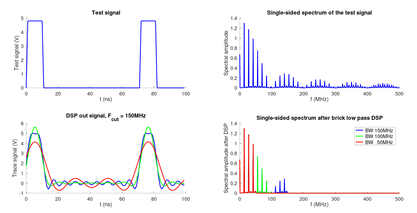
Note the Gibbs artifacts that only a DSP can give. For example, looking at the blue 'Trace signal (V)' right before the raising edge, there is a fake dip in the blue trace wiggling. This type of artifact is impossible to have in an analog oscilloscope/amplifier, even in an overshooting one, because the analog trace can not know when a new rising edge will come (so to wiggle down in anticipation).
The LTspice simulation (of an analog oscilloscope) clearly do not show any DSP wiggling artifacts no matter the BW.
Similarly, note how the green 'Trace signal (V)' in the DSP filtering have a big overshoot above the blue trace, and it is higher than the original signal of max. 4.8V. Such artifacts would be impossible to see in an analog oscilloscope. In digital oscilloscopes, turning sin(x)/x interpolation on might alleviate these kind of issues, but not remove them completely.
Such an overshoot is not possible to have in an analogue oscilloscope/amplifier with Gaussian response, and the LTspice simulation indeed does not show any overshoots.
One may wonder how come that a DSP might have a "premonition" and know to wiggle more right before a raising edge, can a DSP guess the future?

No, it can not. It just works with batches of samples (has memory, Fourier transform can not be made sample by sample, it can only be applied on batches of signal), so the wiggle (and the edge) displayed by the trace are delayed relative to the input signal.


