I ran a test that recorded the phase difference between my Rubidium oscillator (FEI FE-5650A) and a cheap GPSDO I bought on ebay, which is described in the discussion within
this thread. Internally, it is identical to the unit shown
here. The phase difference data described below was collected after both the Rubidium oscillator achieved Lock and the GPSDO showed satellite acquistion and oscillator integrity whereby the accumulated frequency error was less than 100 mHz (the latter condition occurs when the ALM LED goes off, see
the ebay listing). After that condition arose, I waited an extra hour for complete oscillator warm-up before viewing signals and collecting data. For the purposes of this micro-study, I assumed the GPSDO was the reference clock and the Rubidium oscillator was the DUT. To minimize noise in the scope probe measurements, I didn't use the normal ground wire configuration. Instead, I used the spring on the probe tip technique, which meant the distance between the probe tip and grounding site was on the order of a few mm.
I obtained the phase difference data using an ebay board hosting an AD8302 chip (
data sheet here). Characteristics of this chip important to this discussion are: 1) it provides both an amplitude and phase difference signal. The phase difference signal is free from oscillator AM modulation noise.
The AD8302 phase difference signal encodes the phase difference as a voltage, where the phase difference runs from 0 - 180 degrees (180 - 360 degrees is mapped onto that interval with
decreasing increasing voltage). 180 degrees of separation is represented by 30 mV; 90 degrees of separation is represented by 900 mV; and 0 degrees of separation is represented by 1.8V. Therefore, 10 mV excursion represents 1 degree of change. There are dead zones near 180 and 0 degrees.
The AD8302 uses a multiplier circuit to detect phase changes. It turns out that when comparing 2 10MHz signals, the sum of these frequencies leaks through (i.e., there is a 20MHz component). The AD8302 provides for lowering the output bandwidth by adding an external capacitor. For the tests described below, I used a 68pf capacitor, which is insufficient to suppress all of the 20 MHz (and, it turns out 40 MHz) signal.
Figure 1 shows the spectral power density of the phase difference signal from 1 - 100 MHz.
Figure 1 -

Figure 2 shows the spectral power density from 9 KHz-1 MHz. As is evident, most of the spectral power density exists between 0 Hz and 400 KHz. The power below 9 KHz is not analyzable by my SA (a SIGLENT SSA3021X).
Figure 2 -

Figure 3 shows the oscilloscope display (Rigol DS 1104Z) of a typical phase difference signal.
Figure 3 -

Figure 4 shows a zoomed-in display of the 20 MHz signal modulated on the phase difference signal.
Figure 4 -

I ran a one-shot capture of the phase difference signal and moved it to a USB stick. Important parameters for the data series are: 500 Msa/s and 6 Mpoints captured - implying 2 ns between each data point and a 12 msec (2ns * 6E6) capture period. After importing the data into Octave, I ran a 5th order Butterworth 10 MHz low pass software filter on it to eliminate the 20 MHz modulation. Figure 5 shows 100,000 points of the filtered data (in black) superimposed over the unfiltered data (in yellow).
Figure 5 -

The data set exported by the Rigol has two columns: 1) the index of the row (i.e., 0, 1, 2, 3, ....) and the voltage for that data point. I converted the index column into a time value by multiplying it by 2*10e-9 and converted the voltage value to radians by multiplying each value by ((2*pi)/360)/.01. Figure 6 shows the resulting data set.
Figure 6 -
 Corrected Figure 6, which didn't have full x-axis label.
It is apparent from this figure that the data set contains significant white noise. I used the dftmag2 Octave (and MATLAB) function described in the (excellent) article
Real spectrum analysis with Octave and MATLAB to create a spectral density plot of the software filtered phase difference data. This function eliminates the DC (first bin) and last bin values, since (as explained in the article) they must be normalized differently than the other data and there is no normalization procedure that works well. Figure 7 shows the result (using a loglog plot).
Figure 7 -
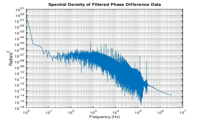
Several features are notable. First, comparing the plot with Figure d on pg. 75 of the report
Handbook of Frequency Analysis by W. J. Riley, it appears that the signal is composed of white noise at frequencies greater than 1000 Hz. However, between 10Hz and 1000Hz, the loglog plot has an average slope of zero. From 1Hz to 10 Hz the slope is very steep. I am insufficiently schooled in phase fluctuation analysis to interpret the last two characteristics.
There is one other interesting result. I wanted some sense of the variation of phase differences over the 12 msec interval. The max and min of the raw data are 0.74100 and 0.55700 respectively. Converting this to degrees (which are easier to visualize than radians) yields 74.1 and 55.7, which is a difference of 18.4 degrees. This is an enormous variation of phase between the DUT and Reference Clock for such a short interval of time, which took me by complete surprise. This may indicate a problem with my test setup or may suggest that the very short-term stability of the Rubidium and GPSDO oscillators are horrible. Recall that both utilize a crystal oscillator in a frequency locked loop. It may be that the feedback loop frequency is significantly greater than 12 msec, which allows the crystal oscillator to display significant jitter during short intervals. However, this result completely mystifies me.
I am new to oscillator evaluation and freely acknowledge that my test setup and analysis may have significant flaws. I welcome any constructive criticism that others might give. I also have made the data I collected available for others to inspect or analyze. The zipped cvs file is available
here. At the beginning of the file is a Creative Commons Share-alike/Attribution license as well as some comments, which means effectively you can do anything you want with it. Each line of text has the "%" character in the first position, so the file can be loaded by Octave or MATLAB without change. For other analysis engines, it is up to the user to convert the file to the appropriate format.


